SST Anomaly

Figure: Global maps of sea surface temperature anomalies (ºC) for the latest month. Anomalies are with respect to 30-year mean OISST.

Status of EL Nino / La Nina

NiNO 12

Figure: Sea Surface Temperature anomalies (ºC) of NiNO 12 (10°S-0°N & 90°W-80°W) region.

NiNO 3

Figure: Sea Surface Temperature anomalies (ºC) of NiNO 3 (5°S-5°N & 150°W-90°W) region.

NiNO 3.4

Figure: Sea Surface Temperature anomalies (ºC) of NiNO 3.4 (5°S-5°N & 170°W-120°W) region.

NiNO 4

Figure: Sea Surface Temperature anomalies (ºC) of NiNO 4 (5°S-5°N & 160°E-150°W) region.

Figure: Depth-longitude section of the (5ºS–5ºN) region averaged temperature (ºC) for the latest month for the Pacific Ocean longitudes.
The continuous black line represents the mixed layer depth, and the dashed black line indicates thermocline depth (20°C isotherm).

Figure: Depth-longitude section of the (5ºS–5ºN) region averaged temperature anomaly (ºC) for the latest month for the Pacific Ocean longitudes.
Anomaly is computed with respect to WOA09 monthly climatology.
The continuous black line represents the mixed layer depth, and the dashed black line indicates thermocline depth (20°C isotherm).

Status of Indian Ocean Dipole (IOD)

Indian Ocean Dipole Index based on INCOIS-GODAS SST analysis and Monthly climatology of OISST (Reynolds sst;constructed using 1981-2010 data).

Figure: Indian Ocean Dipole mode Index (DMI). The DMI is defined as the difference between the SST anomalies (ºC) of Western (10ºS-10ºN & 50ºE-70ºE) and Eastern (10ºS-0ºN & 90ºE-110ºE) Equatorial Indian Ocean regions (WEST-EAST).

SST and SST anomalies over different regions of IOD for the last 12 months:

Figure: Depth-longitude section of the (10ºS-0ºN) region averaged temperature (ºC) for the latest month for the Indian Ocean longitudes.
The continuous black line represents the mixed layer depth, and the dashed black line indicates thermocline depth (20oC isotherm)..

Figure: Depth-longitude section of the (10ºS-0ºN) region averaged temperature (ºC) anomalies for the latest month for the Indian Ocean longitudes.
Anomaly is computed with respect to WOA09 monthly climatology.
The continuous black line represents the mixed layer depth, and the dashed black line indicates thermocline depth (20oC isotherm).

Artificial Intelligence/Machine Learning

Introduction

Monthly climatological maps of ML-based high-resolution (1/12°) surface pCO2 for the Bay of Bengal ​

The increasing anthropogenic activities have led to the rise of carbon dioxide (CO2) in the atmosphere. The constant rise in this atmospheric CO2 in the ever-changing climate may lead to hazardous effects on human health. Ocean has played a key role in modulating this atmospheric CO2. The ocean surface through gas exchange absorbs or emits CO2. The amount of CO2 in a liquid or gas environment is often referred to by its partial pressure. This partial pressure of CO2 is abbreviated as pCO2. The mathematical sign (positive/negative) of the difference between the atmospheric and ocean surface pCO2 shows whether the ocean is absorbing (positive difference) or emitting (negative difference) CO2. The amount of CO2 absorbed or emitted by the ocean is quantified as air-sea CO2 flux. The Bay of Bengal (BoB) has unique physical characteristics compared to other world ocean basins. BoB receives high freshwater influx from rivers and precipitation. The reversing coastal currents due to the seasonal reversing winds play a vital role in changing the physical and biogeochemical characteristics of this basin. Understanding the spatial and temporal variations of the sea-surface pCO2 for the BoB has been limited due to the unavailability of sufficient observations. The limited number of observations results in high prediction errors in the machine learning (ML) based available products for the BoB. Using a significant number of open and coastal ocean pCO2 measurements and collocated variables controlling pCO2 variability in the BoB, an ML-based high-resolution (1/12°) climatological data product (known as INCOIS-ReML) has been developed, which provides sea-surface climatological (mean state) pCO2 maps and associated air-sea CO2 fluxes for the BoB. The capability of INCOIS-ReML has been demonstrated by comparing it with sea-surface pCO2 data from the BoB Ocean Acidification mooring-based observations and gridded Surface Ocean CO2 Atlas (SOCAT) data. INCOIS-ReML has been found to be performing better than six widely used ML-based pCO2 data products. The high-resolution INCOIS-ReML captures the spatial variability of pCO2, and associated air-sea CO2 flux compared to other ML products in the coastal BoB and the northern BoB. This data product is expected to help the researchers to distinguish the source/sink behavior of the BoB, which essentially improves the Indian Ocean carbon budget in a changing environment.

Figure: Climatological monthly variability of the sea-surface pCO2 produced by INCOIS-ReML.
The climatological reference year for this dataset is 2015.

List of Publications

• Joshi, A. P., Ghoshal, P. K., Chakraborty, K., & Sarma, V. V. S. S. (2024). Sea-surface pCO2 maps for the Bay of Bengal based on advanced machine learning algorithms. Scientific Data, 11(1), 384.

ENSO Outlook

Early forecasting of the El Niño Southern Oscillation (ENSO), one of the most prominent climate modes, is highly desired due to its significant impact on the socio-economic health of nations across continents. ENSO is closely linked to slow oceanic variations and their interactions with the atmosphere, indicating the potential for early prediction. ENSO has substantial physical connections to slowly evolving oceanic elements in various regions, including the tropical Pacific Ocean, Indian Ocean, Atlantic Ocean, Western Hemisphere warm pool, and North Pacific Ocean, even at extended lead times. This suggests that improved representation of these interconnected regions and teleconnections in dynamic or statistical models could enhance the long-term predictability of ENSO. However, the irregular amplitude and periodicity of 2-7 years, along with the complexity and nonlinearity of the ocean-atmosphere interactions that generate ENSO, limit the extent of its extended predictability.
Our ENSO outlook is inspired by Ham et al. (2019), who demonstrated that using a convolutional neural network (CNN) model with sea surface temperature (SST) anomaly and ocean heat content (OHC) anomaly as predictors could achieve a lead time of about 17 months in ENSO forecasting. A significant drawback of these deterministic systems is their inherent inability to estimate forecast uncertainty. To address this gap, we employ Bayesian Convolutional Neural Networks (BCNNs), a probabilistic method that leverages the advantages of CNN models while also providing uncertainties associated with ENSO forecasts. Unlike traditional neural networks that provide point estimates, BCNNs learn probability distributions, allowing them to effectively measure uncertainty.
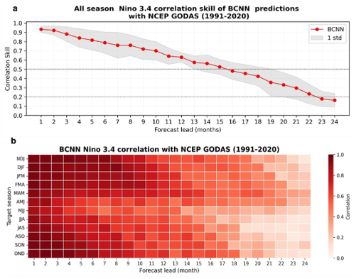
We use globally gridded monthly sea surface temperature anomaly (SSTA) data and vertically averaged ocean potential temperature anomaly for the upper 300 m (VATA) data, both at a resolution of 2.5°x2.5°, covering 0°-360°E and 55°S-60°N for three consecutive months (n, n-1, n-2) as predictors of ENSO. The predictand, or target, is the three-month averaged Niño3.4 index, represented by the difference in area-averaged SSTA over 170°W–120°W and 5°S to 5°N. The BCNN model is trained using monthly SSTA and VATA data from 1871-1980, sourced from 11 models in the Coupled Model Intercomparison Project (CMIP) phase 5 (CMIP5), 14 CMIP6 models and Simple Ocean Data Assimilation (SODA) reanalysis. Only CMIP models that reasonably reproduce ENSO features are selected. The BCNN model exhibits a good prediction skill of more than a year especially for fall, winter and early spring target months. However, the skill exceeding 0.5 during late spring and monsoon extends to about 9 months. This study augments the data used in Ham et al. (2019), which only utilised CMIP5 models.
INCOIS uses predictors from INCOIS-GODAS model analysis to provide the ENSO outlook.

Table 1: List of CMIP6 and CMIP5 models used for BCNN training along with the respective skills (Hou, M. & Tang, Y., 2022 ) in reproducing ENSO.

(a) All-season correlation skill of BCNN compared with NCEP-GODAS (1991-2020). Gray shading shows one standard deviation.
(b) Skill score: seasonal correlation skill of BCNN compared with NCEP-GODAS (1991-2020).

List of References

• Ham, Y. G., Kim, J. H., & Luo, J. J. (2019). Deep learning for multi-year ENSO forecasts. Nature, 573(7775), 568–572.    https://doi.org/10.1038/s41586-019-1559-7
• Hou, M., & Tang, Y. (2022). Recent progress in simulating two types of ENSO–from CMIP5 to CMIP6. Frontiers in Marine Science, 9, 986780.    https://doi.org/10.3389/fmars.2022.986780
• Sreeraj, P., Balaji, B., Paul, A., & Francis, P. A. (2024). A probabilistic forecast for multi-year ENSO using Bayesian convolutional neural network. Environmental Research Letters, 19(12), 124023.    https://iopscience.iop.org/article/10.1088/1748-9326/ad8be1/

ENSO Outlook Bulletin

S.No	Description	Report
1	Outlook of NINO 3.4 index for the period February 2026 - October 2026