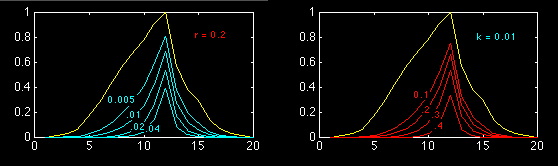
A theoretical example for concentration distributions of a non-conservative pollutant. The estuary is assumed to consist of 20 compartments with constant r. The pollution outlet is located in compartment 12. The yellow curves show the concentration distribution for a conservative pollutant.

The figure on the left assumes a constant ratio r = V_f/R = 0.2 and varies the decay constant k from 0.005 to 0.04 or 0.5% to 4% of one tidal cycle (the cyan curves). The figure on the right assumes a decay constant of 0.01 and varies the ratio r from 0.1 to 0.4 (the red curves). The concentration of the pollutant is reduced relative to the distribution of the conservative pollutant. Note that the effect is present even in the compartment that contains the outlet, because non-conservative decay sets in while the pollutant is still mixed in that compartment.

contact address: